By David Miller | Spring 2026 – Volume 16

Introduction

If you live in Madison, you will certainly have heard the
phrase “housing crisis” in recent years. You may have also
noticed the near-constant development of new apartment
buildings downtown. This might be related to the over
8,500 first-year students admitted yearly by the University
of Wisconsin – Madison (University of Wisconsin –
Madison and Data, Academic Planning & Institutional
Research 2025). It could also be a result of Madison’s
consistent year-over-year population growth rate of 1.5%,
increasing to 2.8% from 2020 to 2023 (Department of
Planning & Community & Economic Development 2025).
Regardless of the reason, Madison continues to grow, and
the talk of a housing crisis persists. As pressure builds,
policymakers and citizens alike begin to second-guess the
1966 statute limiting building height.

Madison’s Height Restriction

Despite Madison’s continued development, we haven’t yet
seen the skyline graduate to that of a major city. That’s
because no matter how high the demand for housing
grows, there is a state ordinance preventing Madison’s
skyline from taking off. Put into place in 1966, the State
Capitol View Preservation statute prevents new
construction 1032.8 feet above sea level within a 1-mile
radius surrounding the Wisconsin State Capitol Building
(State Capitol View Preservation 1990). This raises
concern, as strict zoning laws are associated with higher
rents (Glaeser and Gyourko 2002; Stacy et al. 2023). This
isn’t surprising, as a regulation that limits where and how
housing can be built would artificially constrain the
housing supply. The good news is that any newly built
housing, even housing that isn’t specifically “affordable,”
loosens the market for low-income renters (Mast 2023).
The height restriction in Madison is important for a
variety of reasons, but this paper will focus on housing
density.

Why Housing Density Matters

The effects of a higher housing density are a
contentious topic. Denser housing has been shown to
cause increased economic activity, such as higher
income growth and higher wages (Ahlfeldt and
Pietrostefani 2019; Hummel 2020). It is also associated
with more physically active citizens (Frank et al. 2005).
At the same time, it is correlated with lower greenhouse
gas emissions, lower carbon emissions, and lower
energy use throughout a building’s life cycle (Norman
et al. 2006; Clark 2013). However, the social effects are
more mixed. Higher density was connected to greater
social interaction with friends, but decreased social
interaction with neighbors (Hawley 2012).
Furthermore, several studies have reported that people
prefer to live in lower density areas (Gyourko and
McCulloch 2024; Gordon and Richardson 1997).
Together, these findings illustrate the varied and
meaningful effects of housing density, making it an
important metric for urban policy.

What We Expect Cities to Look Like

One of the most popular theoretical models of a city is
the Alonso-Muth-Mills Monocentric city model. In
this model, housing is allocated through a marketclearing
rent. Commuting is costly, so individuals must
decide to live close to the Central Business District
(CBD) and pay higher rents, or save on rent but
commute longer distances. This model is a vast
oversimplification, but it provides benchmarks for
comparison with real-life cities. Namely, the model
predicts that housing prices, building height, and
housing density increase as one moves closer to the
CBD (Brueckner 2011).

Methodology

To study the distribution of housing density and rents
across a city, one would need spatial data with
information about where people live and how much they
pay in rent. Thankfully, all of that data is publicly
available through the United States Census and
American Community Survey (U.S. Census Bureau 2020;
U. S. Census Bureau 2021).

Analysis will be conducted using data from a 3-mile
radius around the Capitol of each city. A 3-mile radius
was selected because it contains enough data for analysis
while avoiding potential effects from nearby suburbs.
Fitchburg and Middleton, for example, may act as
alternative CBDs which would attract residents. This
study is intentionally focused on Madison, so these
effects are unwanted.

I chose Austin and Lansing as comparison cities because
they are similar to Madison in a few key ways: they are
both state capitols with university campuses downtown.
Lansing is a more accurate comparison to Madison, as it
is a Midwest city with a similar climate and total
population. Austin is less accurate due to its different
climate, much larger total population, and geographic
location. However, it will become useful to contrast
Madison with a much larger city later.

Results and Discussion

First, to assess whether the height restriction has a
significant impact on housing density, I performed a
regression discontinuity. A regression discontinuity is
used when there is a distinct cutoff that divides a treated
group from an untreated group. The idea is that even if
there is a relationship between density and distance from
the CBD, the difference between the density at 1.01 and
0.99 miles away from the Capitol shouldn’t be that
significant. That is, unless there was some other effect
influencing the housing density at that specific boundary.
This is what a regression discontinuity design tests.

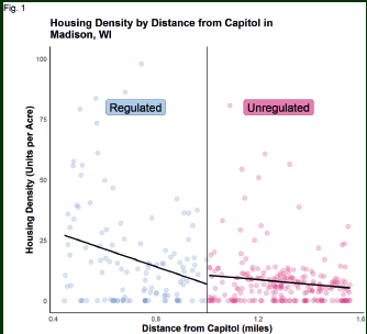
The estimated discontinuity is sensitive to bandwidth,
suggesting limited evidence that the height restriction has
a causal impact on density at the edge of the radius. This
means that there isn’t a significant effect at the policy
threshold, but the height restriction could still be binding
housing density somewhere within the radius.

The estimated discontinuity is sensitive to bandwidth,
suggesting limited evidence that the height restriction has
a causal impact on density at the edge of the radius. This
means that there isn’t a significant effect at the policy
threshold, but the height restriction could still be binding
housing density somewhere within the radius.

Alternatively, one might expect that at the edge of the
height restriction, there may not be a sharp jump in
housing density, but instead a change of slope. Instead of
housing density continuing to grow as it approaches the
Capitol, the restriction may slow or stop its growth.
Similar to the regression discontinuity, the estimated
change in slope is insignificant and sensitive to the
bandwidth, suggesting limited evidence that the height
restriction has a causal impact on the rate at which
density changes with respect to distance from the CBD at
the edge of the radius.

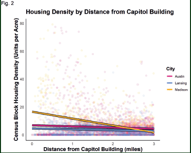
To get a reference, it is worth comparing Madison to
similar cities without a height restriction. The distribution
of housing density, measured as housing units per land
acre, against distance from the State Capitol Building in
each Madison, Austin, and Lansing, is plotted to the right
(Fig. 2). For readability, values above 80 units per acre are
excluded, but the regression results include all values.

For each mile further from the Capitol, Madison’s
housing density is expected to decrease 5.02 units per acre
faster than Austin’s, and 6.35 units per acre faster than
Lansing’s on average. Additionally, zero miles from the
Capitol, Madison is expected to be 12.13 units per acre
more densely populated than Austin, and 16.89 units per
acre more densely populated than Lansing. This is
significant because Austin has a significantly higher
population than Madison, yet Madison has a higher
housing density.

Similarly, we can compare the gradient of median rent for
census tracts against distance from the Capitol for each
city (Fig. 3).

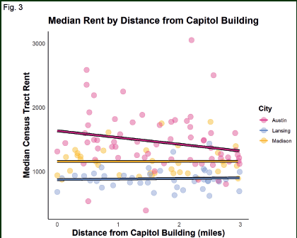
For each mile away from the Capitol, the median rent
change is not significant in any city. Furthermore, zero
miles from the Capitol, Austin’s median rent is expected
to be $478.8 higher than Madison’s, which is significant at
p < 0.001. This means that the rent in each city is
effectively unrelated to the distance from the CBD, and
Austin has a significantly higher rent level. The Alonso-
Muth-Mills model predicted a decreasing rent, while the
data shows that the rent gradient is flat.

The empirical gradients are flatter than predicted by the
monocentric model, implying that these cities may not
be well-represented by a monocentric market.

One potential explanation for Madison’s
disproportionate housing density is its geography.
Madison’s lakes take up a significant portion of the area
surrounding the CBD. This would explain a higherthan-
expected housing density.

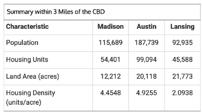
The table above shows that Madison has fewer housing
units than Austin near the CBD. Yet, Madison has a
total average housing density closer to Austin’s than
Lansing’s, the properly sized comparison city. Madison
and Lansing have a similar number of housing units,
with a similar population, but Madison has about half
as much land area as Lansing. This suggests that
Madison’s lack of developable land due to its location
on an isthmus plays a large role in its surprisingly high
housing density.

Limitations

There are several limitations to keep in mind when considering the results of this analysis. First, I chose to use the Capitol building as the CBD for each city. Each Capitol building is placed in the center of downtown, but there isn’t a straightforward way to measure “the center of downtown”. Additionally, these cities may not be monocentric. One could consider the university and the Capitol building in each city as their own CBDs, which would make them polycentric. Lastly, the legislation I am analyzing deals with building height, not housing density or rent. I am relying upon the assumption that a restriction on building height directly restricts housing density.

Conclusion

Performing a regression discontinuity and regression kink on the distribution of housing density against distance from the Capitol building in Madison failed to show that there was a statistically significant discontinuity or slope change at the one-mile boundary of the Capitol View Preservation Order. Despite this, comparing Madison’s housing density gradient to that of Austin and Lansing reveals something surprising. Madison has a similar average housing density to Austin, despite Austin being much more populated. Madison also has a much lower developable land area downtown than in reference cities, suggesting that its geography may impact its uniquely high density. From wages and income growth to physical activity and social connectedness, high housing density has been linked to a variety of important variables central to urban life. Madison residents feel the pressure rising as the sentiment surrounding a housing crisis intensifies. 60 years after the height restriction was put into place, it remains important to question whether it is beneficial.

---

Ahlfeldt, Gabriel M., and Elisabetta Pietrostefani. 2019. “The Economic Effects of Density: A Synthesis.” Journal of Urban Economics 111 (May): 93–107. https://doi.org/10.1016/j.jue.2019.04.006.

Brueckner, Jan K. 2011. Lectures on Urban Economics. MIT Press.

Clark, Thomas A. 2013. “Metropolitan Density, Energy Efficiency and Carbon Emissions: Multi-Attribute Tradeoffs and Their Policy Implications.” Energy Policy 53 (February): 413–28. https://doi.org/10.1016/j.enpol.2012.11.006.

Department of Planning & Community & Economic Development. 2025. “City of Madison Growth Trends.” Madison, WI, December 22. https://www.cityofmadison.com/dpced/housing-initiatives/2025-housing-snapshot-report/growth-trends.

Frank, Lawrence D., Thomas L. Schmid, James F. Sallis, James Chapman, and Brian E. Saelens. 2005. “Linking Objectively Measured Physical Activity with Objectively Measured Urban Form.” American Journal of Preventive Medicine 28 (2): 117–25. https://doi.org/10.1016/j.amepre.2004.11.001.

Glaeser, Edward L., and Joseph Gyourko. 2002. “The Impact of Zoning on Housing Affordability.” Working Paper No. 8835. Working Paper Series. National Bureau of Economic Research, March. https://doi.org/10.3386/w8835.

Gordon, Peter, and Harry W. Richardson. 1997. “Are Compact Cities a Desirable Planning Goal?” Journal of the American Planning Association 63 (1): 95–106. https://doi.org/10.1080/01944369708975727.

Gyourko, Joseph, and Sean E. McCulloch. 2024. “The Distaste for Housing Density.” Working Paper No. 33078. Working Paper Series. National Bureau of Economic Research, October. https://doi.org/10.3386/w33078.

Hawley, Zackary B. 2012. “Does Urban Density Promote Social Interaction? Evidence from Instrumental Variable Estimation.” Review of Regional Studies 42 (3). https://doi.org/10.52324/001c.8101.

Hummel, Daniel. 2020. “The Effects of Population and Housing Density in Urban Areas on Income in the United States.” Local Economy 35 (1): 27–47. https://doi.org/10.1177/0269094220903265.

Mast, Evan. 2023. “JUE Insight: The Effect of New Market-Rate Housing Construction on the Low-Income Housing Market.” Journal of Urban Economics, Special Issue: JUE Insight Shorter Papers, vol. 133 (January): 103383. https://doi.org/10.1016/j.jue.2021.103383.

Norman, Jonathan, Heather L. MacLean, and Christopher A. Kennedy. 2006. “Comparing High and Low Residential Density: Life-Cycle Analysis of Energy Use and Greenhouse Gas Emissions.” Journal of Urban Planning and Development 132 (1): 10–21. https://doi.org/10.1061/(ASCE)0733-9488(2006)132:1(10).

Stacy, Christina, Chris Davis, Yonah Slifkin Freemark, et al. 2023. “Land-Use Reforms and Housing Costs: Does Allowing for Increased Density Lead to Greater Affordability?” Urban Studies 60 (14): 2919–40. https://doi.org/10.1177/00420980231159500.

State Capitol View Preservation, Pub. L. No. 16.842, Stat. (1990). https://docs.legis.wisconsin.gov/statutes/statutes/16/iv/842.

U. S. Census Bureau. 2021. “TIGER/Line Shapefiles.” February 2. https://www.census.gov/geographies/mapping-files/time-series/geo/tiger-line-file.html.

University of Wisconsin – Madison and Data, Academic Planning & Institutional Research. 2025. “Trends in New Freshman Applicants, Admits, and Enrollments in Fall Semesters.” https://uwmadison.app.box.com/s/a6924b0oncjo12hq7kjzdvl6c4yirjob.

U.S. Census Bureau. 2020. “Median Gross Rent (Dollars).” American Community Survey. https://data.census.gov/table/ACSDT5Y2020.B25064?q=median+gross+rent.